Applicability in construction engineering
Ground water flow rates predefine largely predetermine the construction methods and materials used for footings, basement walls, underground constructions and many other in-ground works. The stability of beds and banks of water reservoirs and channels also depends on the filtration in coastal terrain. Factoring the flow of groundwater improves the simulation accuracy of other physical processes in the ground. When distribution of thermal fields takes place in the ground, the convective heat transfer is caused by groundwater flow.
Water is able to flow through the ground because of the presence of pores, which are voids of various diameters and shapes that appear due to the fact that structural elements produced during terrain formation don’t fit flush with each other. The approach for water flow processes simulation differ according to the degree of water porosity and the velocity of water in pores: if the pores are in a saturated condition, the groundwater flow process is simulated based on the Darcy differential equation; water flow in unsaturated ground is described by Richard’s or Brinkman’s equation.
The Darcy equation
Let us consider the Darcy equation in detail. This equation was named after French fluid power engineer, Henry Philibert Gaspard Darcy, and is a second order partial differential equation:
 (1)
(1)
where  – water source,
  , K – coefficient of groundwater flow,
  = m/s;
  – hydraulic head,
  = m;
= m; 
 – nabla operator.
Water flow velocity vector  , according to the Darcy’s law is:
 (2)
(2)
The following boundary conditions are set for equation (1):
1) Boundary condition of the first order  , here
  – hydraulic head given;
2) Boundary condition of the second order  , here
  – water flow through the boundary surface,
  = m/s, and
  – unit outward normal to the surface.
If the boundary condition of the first order is set on the whole boundary, we have the Dirichlet problem for the Darcy equation; if the boundary condition of the second order is set on the whole boundary, we have Neumann’s problem for the Darcy equation. In the general case, we assume that boundary conditions of the first and second order are set at the boundary, and we must therefore consider the problem with mixed boundary conditions.
Due to the arbitrariness of the computational domain, where equation (1) is set, there is no analytical solution for this equation. Therefore, to solve the Darcy equation, numerical methods such as finite-difference approximation of differential operators and the finite element method are used. Here, the first of these methods is considered.
Numerical solution of the Darcy equation
Let the computational domain be a parallelepiped, and the computational mesh of nodes set  . The boundary is the boundary between a material (ground) and the environment as well as the boundary of the computational domain. Each node
  of the computational mesh is assigned vector
  , which is defined the following way:
1)  , if the node
  doesn’t pertain to the boundary;
2) if node pertains to the boundary,  , where
  – components of the normal of the vector in the node .
Let us build the system of equations for numerical solution of problem.  is the approximate value of the head
  in the node . To resolve we build a system of linear algebraic equations. Consider 2 variants according to the geometric location of node . If node doesn’t pertain to the boundary, equation (1) is approximated thus:

If node is located on the boundary, there may be 2 variants depending on the order of the boundary condition set on node. Let the boundary condition of the first order be set on node ; in this case, it is necessary to use  equation. If the boundary condition of the second order is set on node the following equation is used:
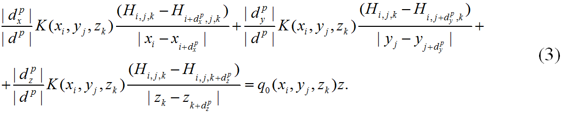
Combining the equations, written for every node of the computational mesh, we obtain a system of linear algebraic equations:
 (4)
(4)
Where the matrix of ![]() coefficients has dimensions
coefficients has dimensions  ,
, .
.
Given that the order of system (4) can be several million for the general case, the system (4) is solved by iterative methods such as the method of simple iterations, the Seidel method, the conjugate gradient method and the biconjugate gradient stabilized method. To accelerate the solution of the system of equations, we use parallel computation on a multi-core CPU and also on a GPU (in particular, CUDA technology is used).
After solving the system (4), the approximate value of water flow velocity vector is obtained through the finite-difference approximation of equation (2) by means of numerical differentiation of the calculated hydraulic head.
During simultaneous simulation of thermal fields and groundwater flow, it is necessary to consider the effect of ground freezing. When the ground is frozen, the pores are filled with ice, thereby reducing the rate of water flow. Assume, that water flow coefficient  for the frozen ground is
  , where
  – ice content in the ground
  , and
, and  – water flow coefficient of the ground thaw at the same point.
The example of the computation of water flow velocities in Frost 3D software
Here is an example of the calculation of water flow velocities, which demonstrates that the consistent account of water flow is essential for modeling thermal fields in the ground.
Let the discussed section of the ground have a parallelepiped shape with the dimensions 15mX10mX10m, we specify it as  (see figure 1). Initially, the ground in the parallelepiped is in the thawed state. There is a hydraulic head
  m, on the left face of parallelepiped P (face
  m); on the right face (
 m) hydraulic head is
  m. Under the head gradient, water flow with the following velocity takes place in the parallelepiped:
 m/s
m/s
Here  – is water flow coefficient.
Assume that in parallelepiped P there is a cylindrical section of ground C with the bottom radius (parallel to plane  )
)  m and height
  m, the center of the cylinder has coordinates (5m,5m,5m). Initially, the ground in this cylinder is in the frozen state. As the ground in section C is frozen, the water flow velocity in this section equals 0.
We determine the distribution of temperature fields in the discussed section of the ground in accordance with the set field of water flow velocities with the temperature value on the left face of the parallelepiped (face m) being  , and the right face being (m)
  . The thermophysical properties of the ground for sections P and C and set in the computation, are listed in the tables 1 and 2. As a result of the computation, we obtain the temperature distribution shown in Figures 2 and 3.

Figure 1 – Computational domain
Table 1. – Thermophysical properties
| Parallelepiped | Cylinder | |||
|
2140000 | 2140000 | ||
|
2140000 | 2140000 | ||
|
1.8 | 1.8 | ||
|
1.8 | 1.8 | ||
| Total gravimetric soil moisture | 1 | 1 | ||
|
1000 | 1000 | ||
| Unfrozen water content |  |
|||
|
0 | 0 | ||
|
0.001 | 0.001 | ||
|
+4 | -4 | ||


Table 2. – Boundary conditions
| Boundary condition of a heat problem | Boundary condition of a water flow problem | |
| face x=0 m | Heat transfer by Newton: temperature +20C, heat transfer coefficient –  |
Hydraulic head – 0.5 m |
| face x=15 m | Heat transfer by Newton: temperature -20C, heat transfer coefficient – |
Hydraulic head – 0.0 m |
| Other faces | Heat flow –  |
Water flow velocity – 0 m/s |

Figure 2 – Distribution of thermal fields in degrees Celsius at a depth of 5 meters after 10 days for the given water flow velocity

Figure 3 – Temperature isolines in degrees Celsius at a depth of 5 meters after 10 days for the given water flow velocity
In reality, water flow velocity in parallelepiped P due to the existence of section C isn’t only equal to 3.33×10⁻⁴ m/s, but also has a complex structure. The distribution of water velocity can be obtained by solving the Darcy equation. We obtain the distribution of water flow velocity fields in Frost 3D software package (Figures 4 and 5) and analyze how the thermal field changes with more precise values for groundwater flow velocities. The obtained computational results are given on Figures 6 and 7.

Figure 4 – Projection of the water flow velocity on X axis (micrometers per second), computed on the basis of the Darcy equation

Figure 5 – Projection of the water flow velocity on Y axis (micrometers per second), computed on the basis of the Darcy equation

Figure 6 – Distribution of thermal fields in Celsius degrees at a depth of 5 meters after 10 days for the given water flow velocity based on the Darcy equation

Figure 7 – Temperature isolines in degrees Celsius degrees at a depth of 5 meters after 10 days for the given water flow velocity based on the Darcy equation
Comparing the results of the thermal field computation with the computation of water flow velocity on the basis of the Darcy equation (Figures 6 and 7), we see that, without any computation (Figures 2 and 3), there is a significant difference in temperature distribution. Particularly critical is the fact that the temperature difference in the same nodes for these computations is more than 10 0C in absolute terms.
Conclusion
In the above article we analyzed the approach of the computation of the groundwater flow, based on the numerical solution of the Darcy equation. This equation is justified for applications involving groundwater seepage.
We have given an intuitive demonstration of how essential it is to consistently factor in water flow when modeling thermal fields in the ground.